Project Title: Movie Revenue Analysis and Prediction with Decision Trees and Regression
Team Members: Thomas Brownlow, Talha Ahsan, Giuseppe Pantalone, Nabiha Ahsan

1. Overview of Project
Films play a large role in generating profit and creating new Intellectual properties for media companies however, a multitude of factors including casting, ratings, release date and genre can play a role in a film’s financial success. Anita Elberse explored the role that stars have in the financial success of a film while Neil Terry and co. discussed the role that a variety of factors such as production budget and critical acclaim played as well.[1][2] Despite having all of this information, the large number of factors involved means it can be difficult for producers to predict how successful a film would be. To explore possible solutions to this problem, we decided to see if we could use machine learning algorithms to predict the success of a film to help come up with better earnings forecasts for films. This could prove invaluable in helping production companies decide investment and marketing for films that they produce. Our plan is as follows:
- Use decision trees/random forests for feature selection to find the features that impact revenue the most
- Use several regression to predict the revenue a movie will produce given its features.
2. Exploration and Visualization of Data
A) Data: Movie Industry, Three Decades of Movies[3]
Features of the data, 18 total
- Budget: Amount spent to produce the movie
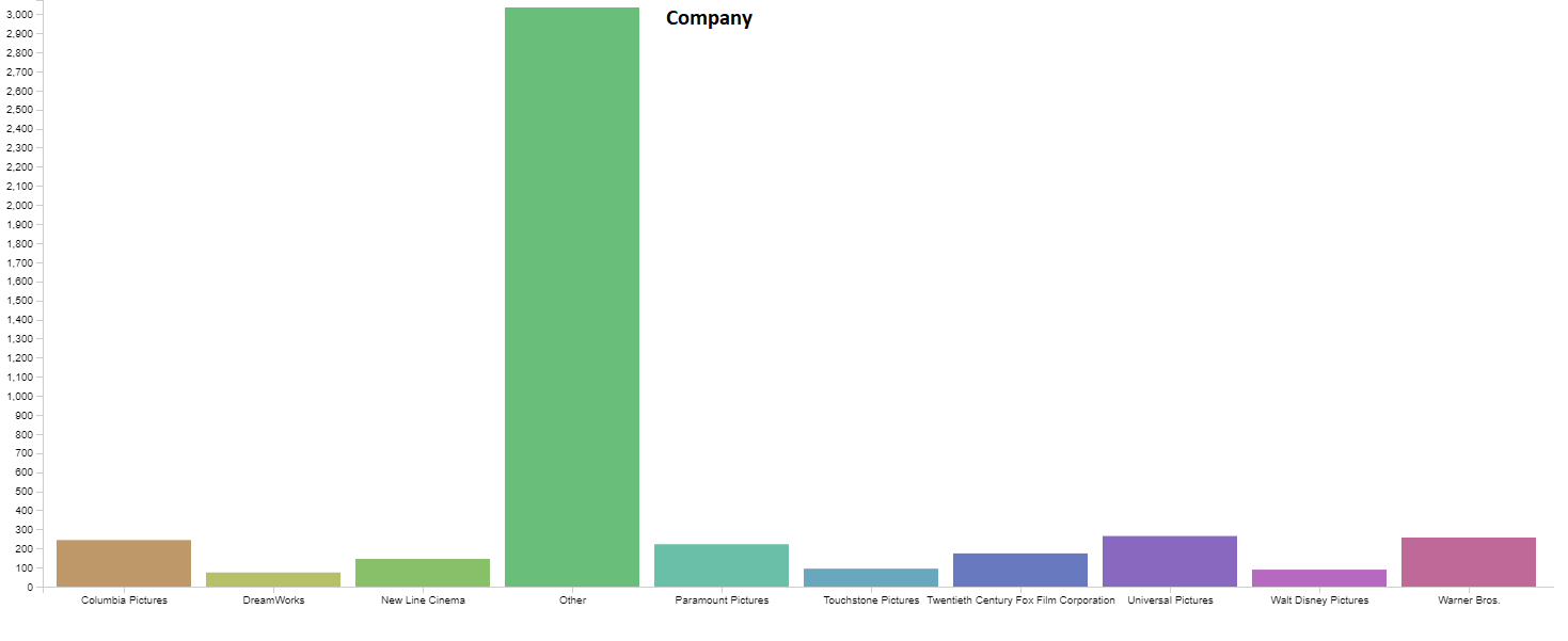
- Company: Production company for the movie
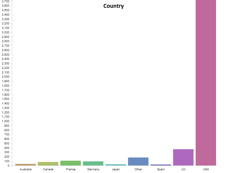
- Country: Country the movie was produced in
- Director: Director of movie
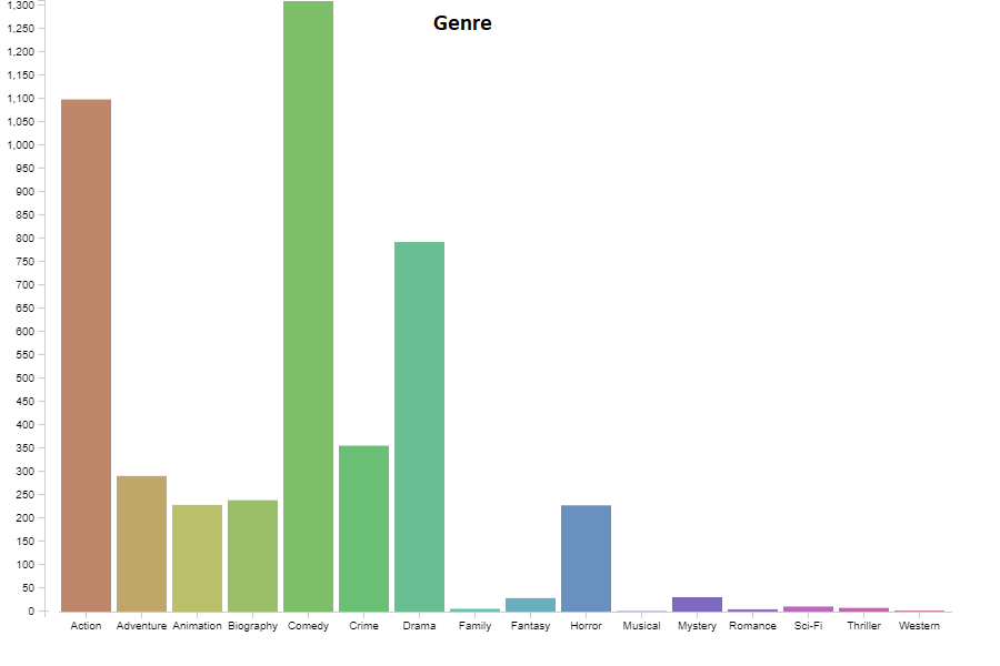
- Genre: Genre of the movie produced
- Gross: Gross revenue of the movie
- Name: Name of the movie
- Rating: Parental Guidance rating of the movie
- Released: Exact release date of the movie
- Runtime: Total runtime in minutes of the movie
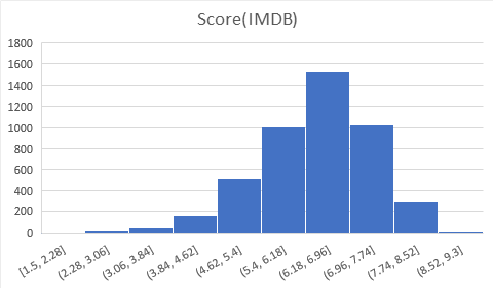
- Score: Score (out of 10) on IMDB
- Star: Leading Actor/Actress for the movie
- Votes: Number of votes (for the score) on IMDB
- Writer: Writer of the movie
- Year: Year the movie was released
- Month: Month the movie was released, a column we derived from release date
- Net Profit: Gross - Budget, also a column we added for each movie
- Profit as % of budget: A feature we created to experiment with predicting. Net Profit / Budget * 100
B) Data Visualization
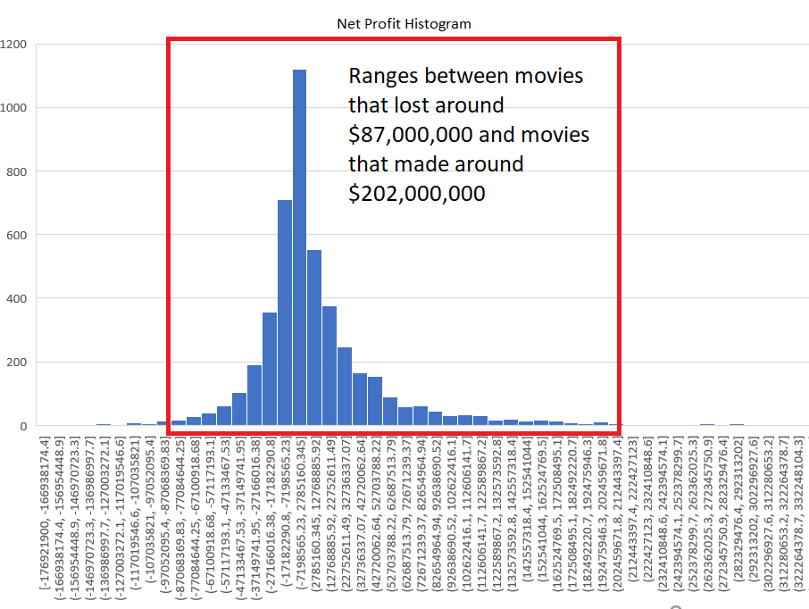
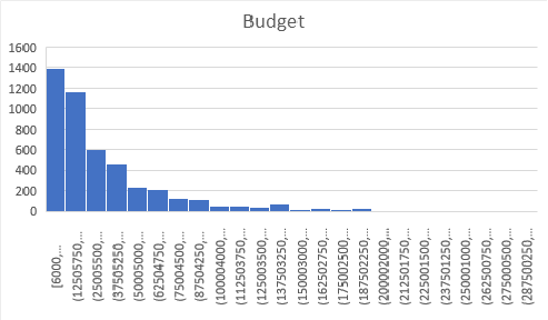
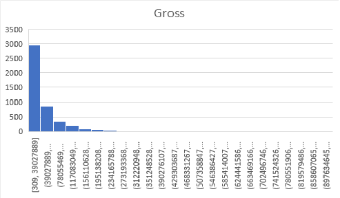
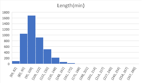
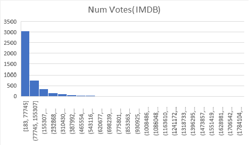
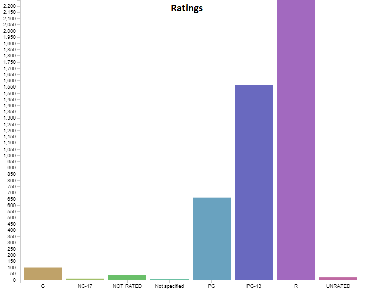
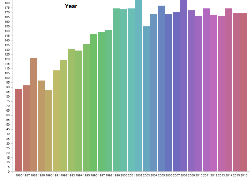
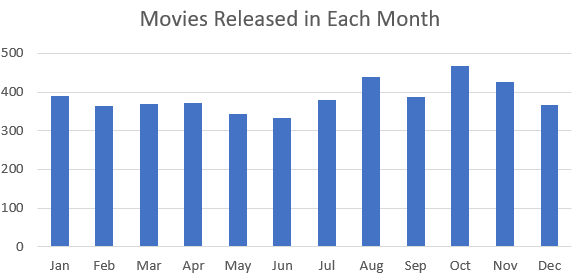
Below are graphs visualizing the distribution each of the features. There are 6820 movies in total, but a decent amount of those have no gross revenue listed which makes them useless for our project. After removing these blank data points we are left with 4638 movies to visualize. You will notice that our features cover of very wide range of values so normalization will be a must. We have continous variables(budget, gross revenue, etc.) and categorical variables(genre, country, company, etc.). There are no graphs for Star, Director, or Writer because these categories are very diverse. Most people only appear once in each of these categories, and at most appear 20 different times. Each of these categories has around 4000 unique entries, out of our 4638 movies total.
3. Data Pre-Processing
After visualizing the data we were able to process the data in some basic ways before we begin features selection.
- As noted above we removed all movies with no gross revenue listed
- Remove repetitve categories (release date is too specific, better to use release month)
- Remove irrelevant to prediction features (movie name, release year) because they wouldn’t be useful to actually predict whether a movie would turn a profit.
- Remove score and votes, which are IMDB values. These features aren’t relevant to our problem. We want producers to be able to predict the revenue of their movie before its made which would be before the movies is reviewed. Other categories like rating, length writer,etc. are decided by them before hand, unlike IMDB stats.
- Normalize the data and use sklearns label encoder for categorical data
4. Feature Selection
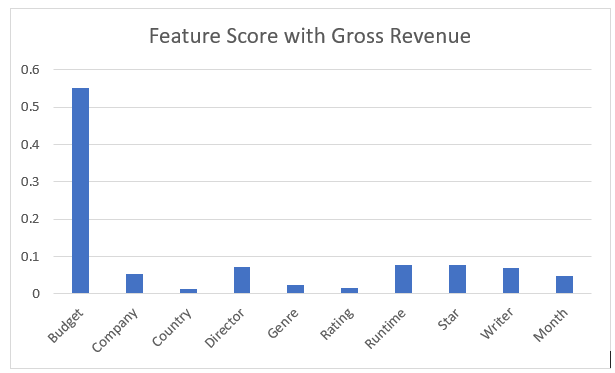
In this section we will explore the methods used for feature selection. First we decided to use random forests to measure the importance of our features. The algorithm measures the decrease in impurity by selecting each feature at a certain branch in the tree. In the regressive case the measure of impurity used is variance. The features which decrese variance the most accross all the decision trees in the random forest will be given a higher importance. Below is a graph of normalized scores which add up to 1.0 (with some rounding). It is recomended to take features that score above the mean. In this case we are measuring 10 features, so the mean is 0.1.
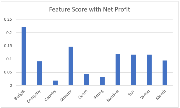
We are predicting for gross revenue, and in this scenario the only recommended feature is budget. Even with normalized features budget is ruling the predictions. In order to create a more stable prediction we decided to try and predict with net revenue instead so that budget wouldn’t rule the prediction. Everyone knows that a bigger budget just makes more money, but does it make enough money? Below is a graph of the exact same thing above, except we use net revenue as the predictor to try and see what other features are important other than budget.
The features that score above 0.1 with this method are Budget, Director, Runtime, Star, and Writer. Company and Year were both very close to the cutoff so we will also experiment with those features. The features that didn’t make the cut are Country, Genre, and Rating.
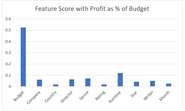
We also decided to take a shot at predicting a metric we came up with called Profit as Percent of Budget. A movie can be successful even if it doesn’t make as much as other movies if it makes a large return on investment. This metric, which we calculated from values in the table is equal to the profit / budget * 100.
It turned out that predicting this outcome relied almost entirely on the budget feature, but for the opposite reason as for gross revenue. Movies that had much smaller budgets tended to be much more likely to have higher percent of budget as profit. Interestingly the only other two categrories that met or were even close to the 0.1 threshold were runtime which met the threshold in predicting other standards, and Genre, which was had one of the lowest feature scores for the other prediction values. It turns out low budget horror movies and comedies tend to be quite profitable as percentages compared to their budget. With some extreme outliers like Paranormal Activity, Blair Witch Project, and Napoleon Dynamite achieving 11,000% and even over 700,000% in the case of Paranormal Activity.
5. Net Revenue Prediction with Linear Regression
The first model we selected to make our predictions was linear regression. We used scikit learn’s linear regression tool to achieve this. We decided to use linear regression as we felt that it fit our use case well since it is useful in predicting continuous values. As we used scikit learn’s tool, the linear regression model we had used Ordinary Least Squares to make estimations. Note that the results were normalized for the sake of this visualization. Due to the large range of values, normalizing was important to make the visualization easier to interpret. We decided to run the model with all the features available and then only with the features we selected above. First up, the results with all the features are shown below:
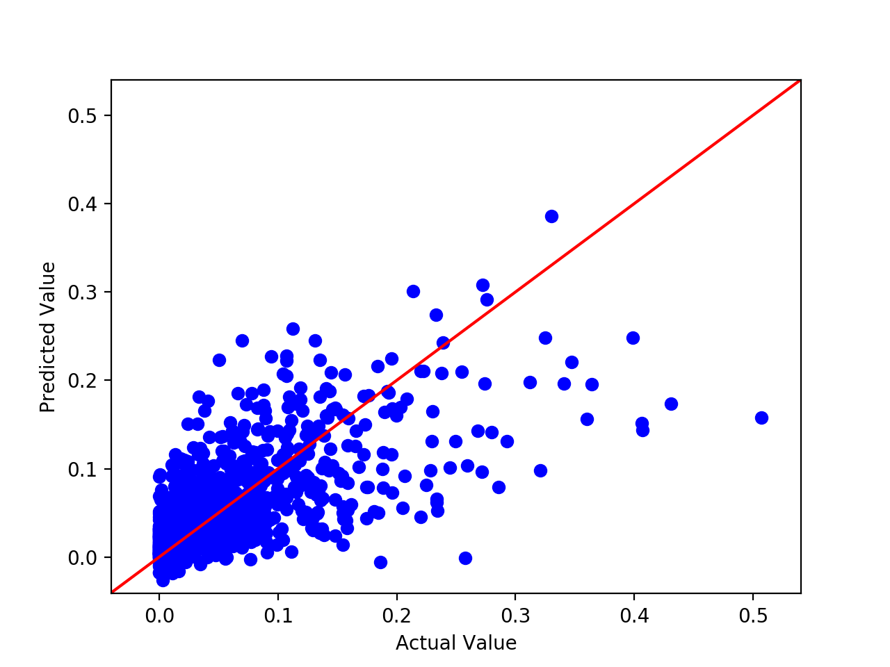
The Root Mean Square Error that we found with all features was 0.0501, and an R^2 of 0.424 indicating that our model had some error in its estimation, but could be improved. Through multiple runs, the RMSE tended to stay around this value. To ensure our model was not overfitting or underfitting, we compared the RMSE value that we received from the training set and the test set. Both RMSE values had very little discrepancy between each other indicating that the linear regression model did not overfit or underfit substantially. As can be seen, in most cases, our linear regression model with all features was quite helpful in at least getting a ball park figure of where a producer could expect the gross of a film to be based on the parameters we chose to include.
We then ran the the same model using only the features we selected above. Country, genre and rating were all dropped to see if that makes any substantial changes to the predictive capabilities of our model. The results of this run are shown below:
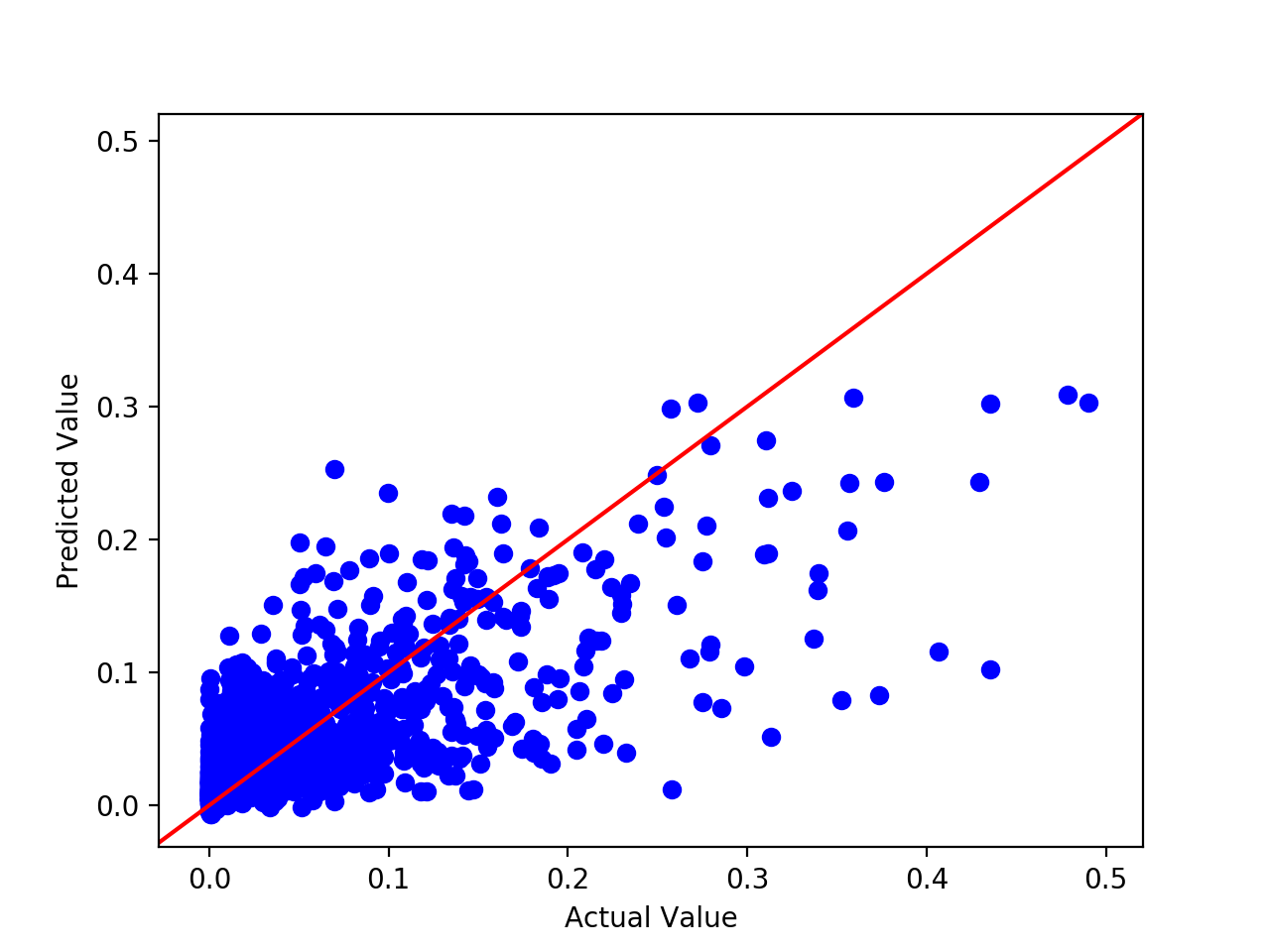
The RMSE we calculated without these three features turned out to be acceptable at 0.04820, and an R^2 of 0.530. Keep in mind that these features are normalized so on a larger scale we would like to get the RMSE to be even smaller as tiny shifts in the value could be important on our scale of millions of dollars.
6. Prediction with Ridge and Lasso Regression
The second and third models we used were ridge regression and lasso regression, again using scikit learn. We used ridge and lasso regression because they are both optimized for prediction. Ridge regression can’t zero out coefficients but in contrast to this, the lasso does both parameter shrinkage and variable selection automatically. Both of these regressions were run with all features.
For our lasso regression model, the Root Mean Square Error that we found was 0.0523. Through multiple runs, the RMSE tended to stay around this value. Once again, to ensure our model was not overfitting or underfitting, we compared the RMSE values from the training set and the test set, and both RMSE values had almost no discrepancy indicating that there was very little to no overfitting or underfitting. Similarly to other models, our lasso regression model with all features was quite helpful in estimating the gross of a film based on our parameters.
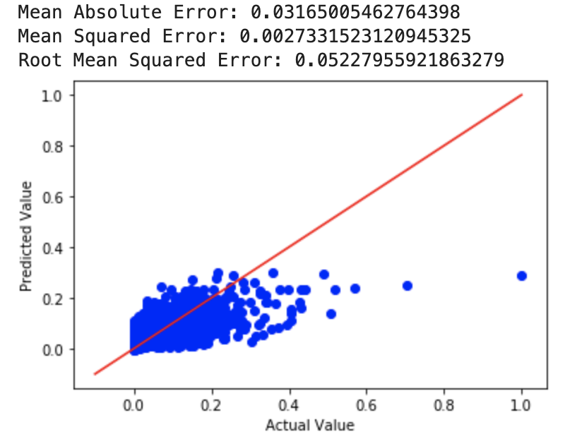
For our ridge regression model, we tried a few different alpha values to see what worked best. We first used an alpha value of 4 and then an alpha value of 10^10. The MSE for a=4 was 0.0650 while the MSE for a=10^10 was 0.0516. Then, we tried it with a=0 (perfomed least squares regression) and got an MSE of 0.0027. After this, we used cross-validation to choose a value of alpha, for which we got an MSE almost identical to that of the least squares regression. The RMSE for the least squares and ridge with cross-validated alpha value was 0.05228.
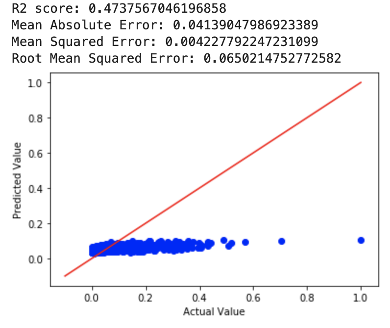
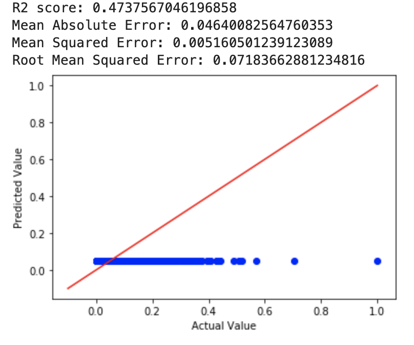
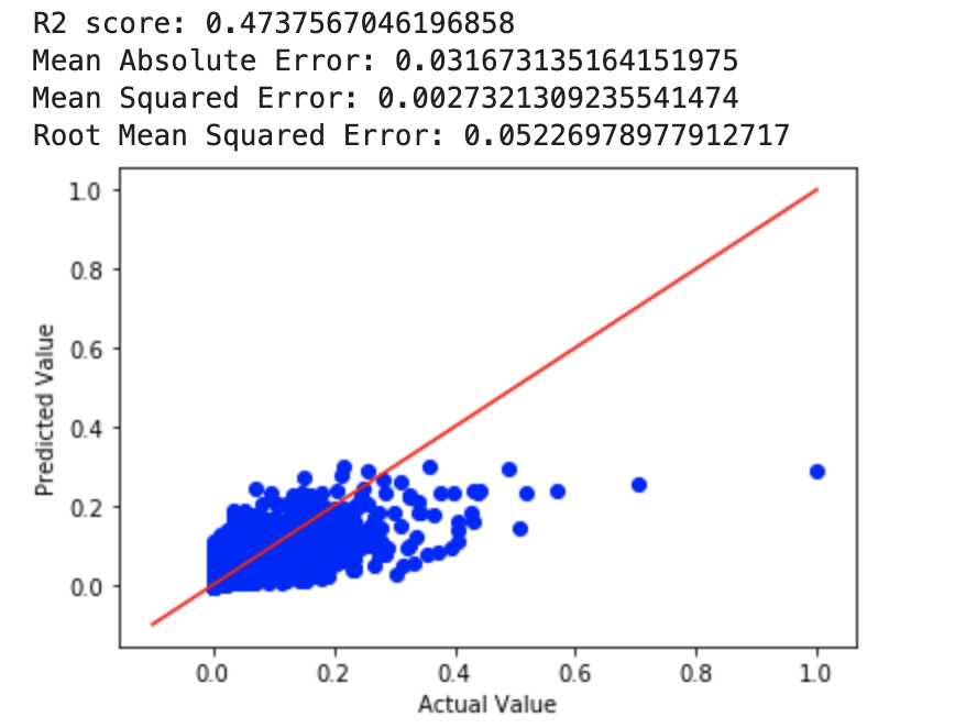
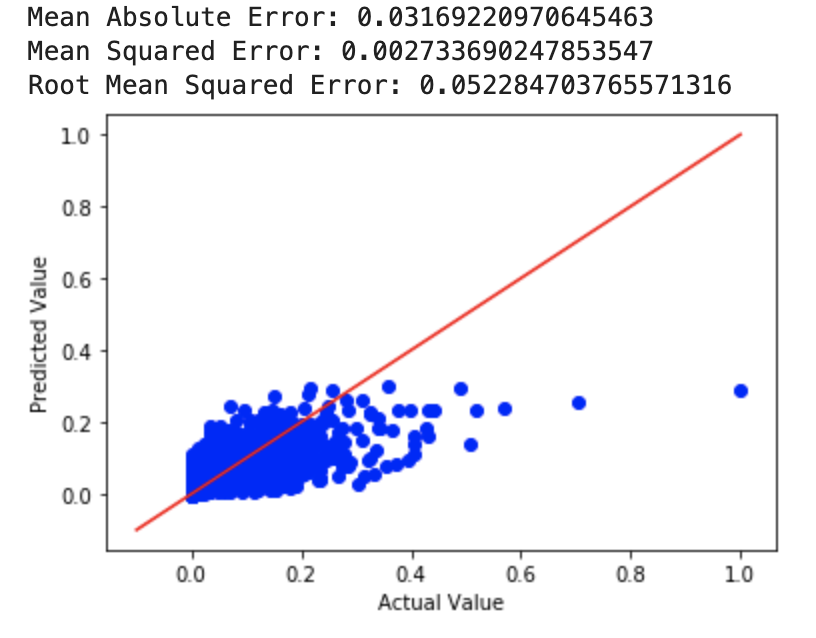
Although the differences in RMSE aren’t huge, the linear regression model outperfomed both ridge and lasso with all features.
7. Prediction with a Neural Network
The fourth model we used was a neural network. We again used scikit learn to implement our model. Specifically, we used the MLPRegressor class to create a neural network. It consisted of 2 hidden layers, each with 32 neurons. Our activation function was relu, and our optimizer was adam. We used an adaptive learning rate and found that performed significantly better than using a constant learning rate. We chose to select a neural network as we felt that the complexity of the problem would likely be handled well by a neural network. The results we received from the model when used with all features are shown below:
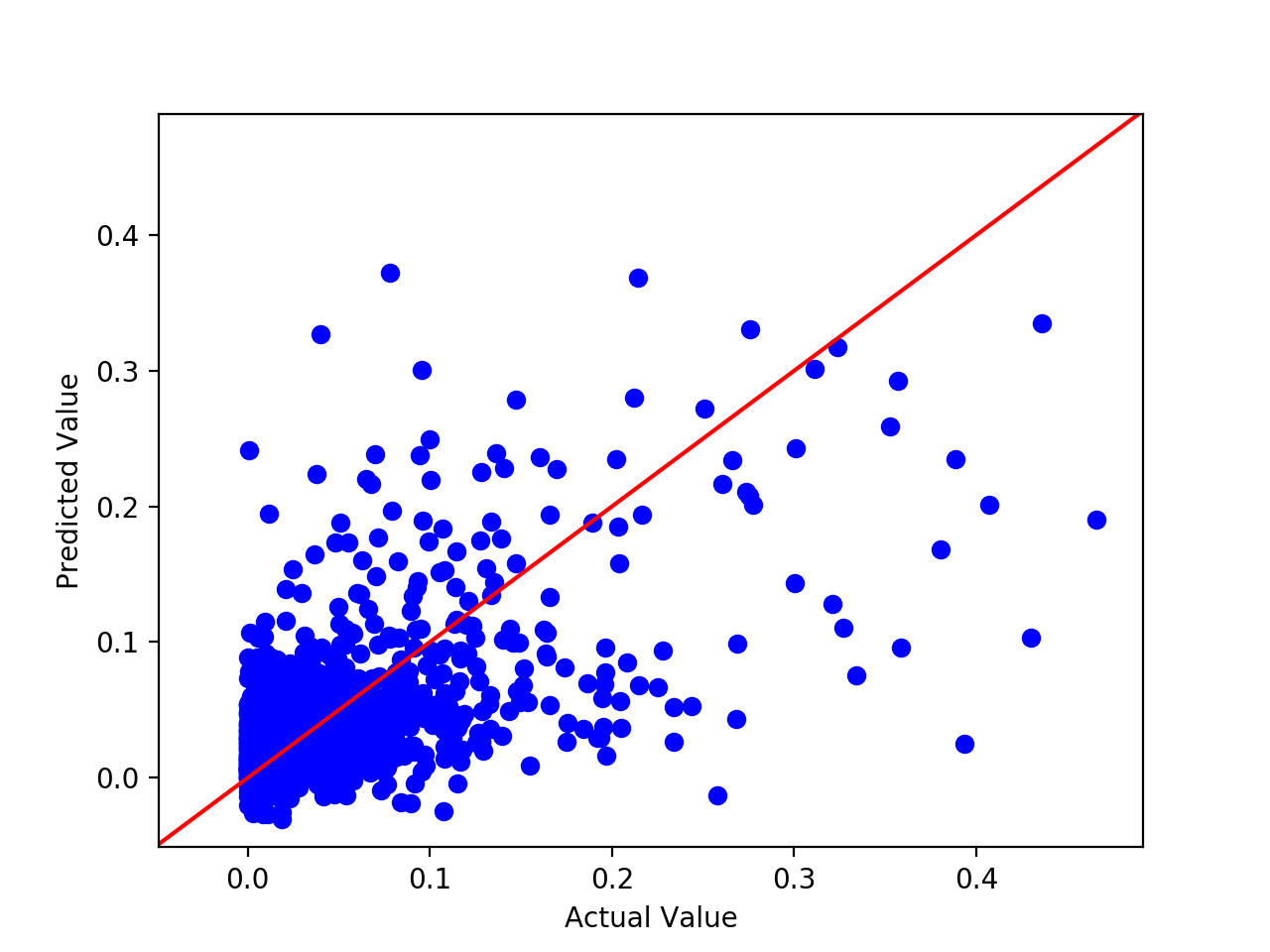
Interestingly, the neural network did not perform better than the linear regression model. As can be seen, the 0.058 RMSE value of the neural network is higher than the observed value from the linear, ridge, and lasso regression models. When used with only the features recommended, the following results were received:
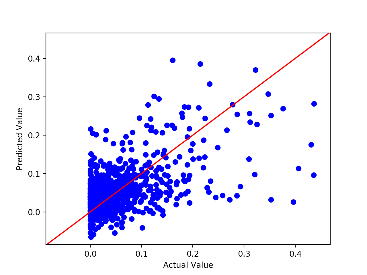
Dropping the extra features showed a slight improvement for RMSE but nothing the massive. The recorded RMSE was 0.054 with the featurese dropped, slightly better than before but still worse than the other models.
8. Conclusion
A) Feature Selection
Using random forests certain helped to narrow down our models to the relevant features, but didn’t provide as much of an impact as we would have expected. We believe this is because of 2 different things. First, no matter whether you look gross revenue, or net revenue, budget dominates the prediction so the other features are overshadowed by budget. Second, some of the recommended features have a high cardinality of unique values. This makes the data for these features like star and director sparse so in order to capitalize on the true power of these features we would need a much bigger data set. Regardless we can confidently say that the features we found (Budget, Director, Runtime, Star, Writer, Company, and Year) have a significant impact on the revenue a movie produces and should try to be incorporated in any model that aims to predict movie revenue.
B) Regression Models
We explored both linear regression models, and neural network models to help solve our regression problem with an expectation that the neural nets would out perform linear regression, ridge regression, and lasso regression because of the nuance of the problem with many different factors affecting revenue, but ended up finding the opposite. While the difference wasn’t extreme, and the neural nets still performed alright, the linear models overall performed better. We believe this divergence from expectation is exactly due to the reason listed in part A). Our neural net wasn’t able to fully capitalize on the nuances that could be available from the high cardinality features, while the linear model was able to capitalize on the heavy importance budget plays on revenue. These 2 factors together allowed for the linear model to outperform the neural net. The linear model consistently provides values that are close to the actual, and hardly ever over or underestimated by alot., where the neural net was more inconsistent.
C) Results
When starting with this project, we knew that predicting the potential gross of a movie would be a complex problem and that it would be difficult for us to completely encapsulate all the factors necessary for such a prediction. With that said though, the results that we received were very promising. We could predict the gross that we would recieve up to an error of around 5% for most of our models. With linear regression, we achieved our best results and could make predictions within 5%. Thus, even though there was still an error to consider, our model at the very least could serve to provide producer an effective tool to estimate how successful a movie might. This could in turn prove essential in deciding important factors for the movie process such as how much to invest in advertising for a film. Furthermore, producers could also use the model to decide things like which month to release the movie on by running our model with different months for release dates and seeing which one returns the highest gross. For this reason, we believe that our model holds significant promise as a tool to help future film productions.
D) Future Work
We feel that our dataset is mostly what held us back from making a very accurate predictive model. The first reason is lack of certain data that we feel would be very good predictors of revenue, and the second is the high number of categorical features in the dataset. We were unable to find any data on how much money was spent on advertising for the movies, how many theaters it opened in, or how long it was in theaters. All these are features we felt would have been strong continuous features in predicting profit of a movie.
The second problem is two-fold. The first being that while we felt the star, production company, writer, and director of a movie are probably features that very much matter in predicting profitable movies, the fact that they were in the dataset as extremely high cardinality categorical features meant that they were limited in their ability to be good for machine learning. As those categories are nominal features (they have no inherent order) encoding them as numerical features with a simple numeric encoder (1:k for each unique value) lead to them having some sort of implied ordered relationship to our regression and neural network models. Ideally, you would encode those features as a large series of 1-hot encoded columns instead, but since those features had cardinalities in the range of 200-2000 different values, one-hot encoding would have lead to a way too extreme increase in the dimensionality of our feature space. We tried to experiment with hashing function encoding but didn’t produce much better results. In the future we would want to devote more attention to research on properly encoding high-cardinality features and designing models that can work well with such data.
If we could have our ideal dataset, we would like one that had a continuous way of representing these categorical features inherently. For example, instead of the name of the star, it could have their social media following at the time of filming (wouldn’t apply to older movies) which is a continuous way of trying to measure a star’s popularity on the profitability of a movie, rather than trying to guess at its impact from just their name. For directors/writers it could be number of presitious filmmaking awards recieved prior to making the movie, or also social media following. Essentially, we believe that the personnel/companies involved in making a movie do have an impact on profit, but that simply their names are not useful enough for machine learning.
8. References
1) Elberse, A. (2007), The Power of Stars: Do Star Actors Drive the Success of Movies? Journal of Marketing 71, 102–120.
2) Terry, N. Buttler, M. De’Armond, D. (2005), The Determinants of Domestic Box Office Performance in the Motion Picture Industry,
       Southwestern Economic Review, 137-148
3) The Movie Database (2017).TMDB 5000 Movie Dataset, (version 2), Web
4) Hale, Jeff. “Smarter Ways to Encode Categorical Data for Machine Learning.” Medium, Towards Data Science, 16 July 2019,                      https://towardsdatascience.com/smarter-ways-to-encode-categorical-data-for-machine-learning-part-1-of-3-6dca2f71b159.
